Why Charts for Manifolds?
A Walk on the Round Side
Unless you’re a member of the flat earth society, we all recognise that the Earth is round. But it’s not obvious - going outside, walking around and touching grass, it certainly doesn’t feel like the Earth is curved. Certainly there are local features that aren’t at all flat - as far as I know, flat earthers do not think mountains and valleys are secretly flat, too - so the “roundness” of Earth is necessarily some kind of averaged statement. Quite literally global! Of course, a quick trip to space verifies this, but how might you demonstrate the Earth’s curvature using purely surface-level observations?
If you’re adventurous, you could just pick a direction and start walking until you loop back around! But circumnavigating the globe isn’t the most practical solution; instead, we’ll attempt to use a little mathematics and save ourselves the trouble.
Suppose you’ve been given an atlas of the world, which marks important landmarks like the north and south poles, as well as “latitude” lines like the equator. Then you might notice it’s possible to form a triangle of the following shape: 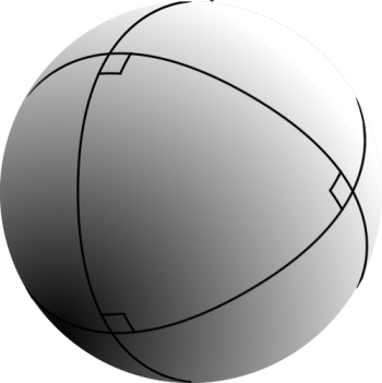
(Source: Spherical Geometry)
Start from the north pole and go “south” in two perpendicular directions (remember that at the north pole, every direction is south!). Keep extending these lines on your map until you hit the equator, and then connect these lines with a purely eastward path.
What we’ve done is make an “equilateral right-angled triangle” - one whose angles are all 90 degrees. This is completely impossible on a flat plane, since the angles of a triangle are supposed to sum to 180 degrees.
There’s a lovely bit of Spherical Geometry called Girard’s Theorem, which relates this “excess angle” beyond the 180 degrees expected for a triangle to its area. So this is an effect that can be observed even for quite small triangles, provided you have extremely precise measuring equipment.
Thus it is possible to deduce the curvature of the Earth as a “global” property through purely “local” means - by considering paths on the surface of the Earth. Even an impractical circumnavigation takes the form of a path around the Earth!
What is a Path?
Paths in a space $X$ are a very important way of “exploring” the space, and this is especially true for manifolds - spaces which are “locally Euclidean” in an appropriate sense. We saw an example of this in the previous section with the sphere $S^2$; much like Earth, the sphere looks “flat” if you can zoom in enough, which lets us transport calculus concepts on $\mathbb{R}^2$ to those on the sphere.
The way paths tend to get formalised is as some kind of continuous/differentiable/smooth function out of $\mathbb{R}$, with a “time” parameter $t \in \mathbb{R}$. We’re familiar with paths in 3D space $\gamma : \mathbb{R} \to \mathbb{R}^3$, given by \(\gamma(t) = (x(t), y(t), z(t))\). It’s straightforward to differentiate this component-wise, obtaining \(\gamma'(t) = (x'(t), y'(t), z'(t))\).
Following the previous example, it’d be nice to consider paths in more general kinds of spaces, like a path on the surface of the sphere $S^2$ given by a smooth map $\gamma : [0, 1] \to S^2$. How would we differentiate it? Say we use a path \(\gamma_0(t) = (\cos(t), \sin(t), 0)\).
Then… it still seems like we can differentiate component-wise, right? We obtain \(\gamma_0'(t) = (- \sin(t),\cos(t), 0)\).
Weirdly enough, we never actually used that the sphere was “locally flat” to demonstrate that our curve $\gamma_0$ was differentiable. All we needed is that the curve had x, y and z components that we could differentiate individually.
Our observation ends up holding true for any subset $S$ of $\mathbb{R}^n$. Paths in $S$ as functions $\alpha : \mathbb{R} \to S$, correspond to functions $\beta : \mathbb{R} \to \mathbb{R}^n$ whose image is contained in $S$, where we have $\beta = \iota \circ \alpha$. Here, $\iota : S \to \mathbb{R}^n$ is the inclusion map, which you can think of as merely “changing the type” of the output. Then $\beta(t) = (x_1(t), \dots, x_n(t))$ to allow us to differentiate “componentwise”.
So, if we’re working with embedded manifolds $M$, as subsets of $\mathbb{R}^n$, we don’t actually need charts to figure out what “smooth paths in $M$” should be! We just need smooth paths $\beta : [0, 1] \to \mathbb{R}^n$ whose image is contained in $M$. Then… what do we need charts for?
Turning up the Heat: Why Local Flatness Matters
Just as important as smooth paths are smooth functions defined on $M$, $f : M \to \mathbb{R}$. For concreteness, say we take $M = S^2$ as a model for the Earth, and we have a temperature function $f : S^2 \to \mathbb{R}$. We want to determine what the “temperature gradient” is.
The multivariate definition comes to mind - at a point $a \in S^2$, we need a linear map $Df(a)$ such that $f(x) = f(a) + D f(a) [(x - a)] + o(x - a)$, using standard Little-o notation. But… what should the dimensions of $Df(a)$ be? We know that it’s supposed to take in a vector $x - a$, and spit out a real number. Since $x - a$ is a 3D vector, it’ll be a linear map $\mathbb{R}^3 \to \mathbb{R}$, represented by a $1 \times 3$ matrix.
Somehow that feels like a bit too much information. The sphere is a surface after all, so there’s only really 2 independent directions. Ideally, we should only need information about the derivative in those directions. This is what our “local coordinates” let us do; in a small patch of the sphere, we can view the temperature function as a map $U \to \mathbb{R}$ for an open subset $U$ of $\mathbb{R}^2$, with the directions representing “latitude” and “longitude”. This allows us to use standard multivariable calculus to get the derivative as a $1 \times 2$ matrix, $\begin{pmatrix} \frac{\partial f}{\partial \theta} & \frac{\partial f}{\partial \phi} \end{pmatrix}$, for $(\theta, \phi)$ angular coordinates, as expected!
This is what charts are built to do for general manifolds - by flattening a patch of the manifold, we can parametrise small changes on the manifold in terms of small changes in flat space, which we know how to differentiate with respect to.
Looking Ahead
Hopefully, what I’ve convinced you of is that:
- To define smooth functions out of a manifold, we need charts to encode displacements on the manifold as displacements in ordinary Euclidean space.
- But for embedded manifolds, charts are not necessary to define smooth functions into a manifold. We simply extend the codomain to $\mathbb{R}^n$ by composing with the inclusion map, and investigate smoothness of that function.
The second bulletpoint is an instance of a general story about “substructures” called the universal property of subobjects:
- If $S \subseteq X$, then functions $Y \to S$ correspond to functions $Y \to X$ whose image is contained in $S$
- If $H \leq G$, then group homomorphisms $Z \to H$ correspond to group homomorphisms $Z \to G$ contained in $H$
- If $E \subseteq X$ for $X$ a topological space, then continuous functions $Z \to E$ (with the subspace topology) correspond to continuous functions $Z \to X$ whose image is contained in $E$
Formalised in category theory, this encapsulates the idea that what a subobject $S$ of $X$ does is let you represent maps $Z \to X$ satisfying some conditions by ordinary maps $Z \to S$ satisfying no additional conditions! Try seeing if you can prove this the next time you come across some kind of substructure :)